RAM Latency VS Clock Speed

You may have noticed that when faster memory first becomes available, it comes with a higher latency than similar existing RAM. Why is this, and how does that affect overall performance? Also, when you overclock RAM in the BIOS, you will get much better results if you adjust the CAS latency at the same time. But how do you know what value to enter for CAS? And what if motherboard limitations require that you use a lower-than-specified RAM speed? Did you know that you then get to use a lower value for CAS?

This article will answer these questions, and includes formulas and charts so you can feel confident in your RAM purchase and use the correct settings.

Summary

You may have noticed that when faster memory first becomes available, it comes with a higher latency than similar existing RAM. Why is this, and how does that affect overall performance? Also, when you overclock RAM in the BIOS, you will get much better results if you adjust the CAS latency at the same time. But how do you know what value to enter for CAS? And what if motherboard limitations require that you use a lower-than-specified RAM speed? Did you know that you then get to use a lower value for CAS?

This article will answer these questions, and includes formulas and charts so you can feel confident in your RAM purchase and use the correct settings.

❗ The latest version of the Excel charts used in this article, including higher memory speeds, will always be available →here←. The header labels will not display correctly in Google Drive, so you must download and display in Excel.

Key

I am using color coding to make the various units stand out. This is especially useful with clock cycle time, which I express in different ways to make its components more clear. All these units are explained in the section titled Clock Cycle Time.

• Red: clock cycle time, ns/T, ns/cycle
• Orange: MT/s
• Green: MHz
• Blue: cycles/ns

Latency

With modern RAM, latency is specified in clock cycles, even though it is really a function of time. If a particular memory stick can’t process a memory request in less than half a nanosecond, that will continue to be true even if you increase or decrease the frequency. So if you increase the frequency, you are decreasing the time of each clock cycle, and that means that you will need more cycles to reach that half nanosecond.

To compare the latencies of memory with different speeds, you need to convert the given latency value to a time value. This will simply be the amount of time it takes for one cycle (clock cycle time) times the number of cycles specified by the latency. Wouldn’t it be nice if manufacturers just gave us that value instead?

Clock Cycle Time

This section gets a bit into the weeds for those who want to feel comfortable with the derivation of the final equation. You don’t need to read this section to understand the charts at the end of this article.

To calculate effective latency, we need to know how long each cycle takes (clock cycle time). We will measure that in nanoseconds (ns), or more accurately, nanoseconds in one transfer (ns/T).

Currently, memory speed is typically measured in Mega-Transfers per second (MT/s). This is actually the data transfer rate, which, for DDR RAM, is double the clock rate. For older SDRAM, the data transfer rate and the clock rate are the same, so they are measured in MHz (million cycles per second).

In calculations in this and the following sections, I will be using these variables:

• D = Data transfer rate in MT/s. For SDRAM, this is the same as clock rate in MHz. For DDR RAM, this is double the clock rate.
• L = Latency as CAS# or CL#. The delay before the contents of the first requested memory column is available in the output, measured in clock cycles for synchronous RAM (all DDR RAM).
• E = Effective latency or true latency in nanoseconds. A lower E is better.

To derive the equation for Clock Cycle Time is to go from MT/s to MHz to cycles/ns to ns/cycle (or ns/T) as in this chart:

MT/s	⇒	MHz	⇒	cycles/ns	⇒	ns/cycles
million transfers per second		million cycles per second		cycles per nanosecond		nanoseconds for one transfer cycle

1. To go from MT/s to MHz for DDR RAM, simply divide by 2, as DDR RAM does two data transfers per cycle. D MT/s = D/2 MHz.
2. To go from MHz (million cycles/s) to cycles/ns, you need to do the following:
   1. Convert million cycles to cycles (go from megahertz to hertz): multiply by 10⁶.
   2. Convert seconds to nanoseconds: multiply by 10⁹.
   3. So, to go from MHz to cycles/ns, multiply top by 10⁶ and bottom by 10⁹ or 1,000,000/1,000,000,000, which simplifies to 1/1000. To include the previous conversion from MT/s in step 1 where we were already dividing by 2, we get D/2000.
3. To go from cycles/ns to ns/cycle, simply invert the equation we have so far. So, we take our original MT/s value (D) and divide by 2000 and then invert to get the clock cycle time. This gives us 2000/D.

Clock Cycle Time = 2000/D

As a side note, the Data Cycle Time for DDR RAM is 1000/D since there are two data cycles for each clock cycle.

True Latency (Effective Latency)

Now that we can calculate the time for one clock cycle, we multiply that by the CL value to get the effective latency. Remember, CL is the number of clock cycles before the first memory word is available.

• E = L * 2000 / D

Since memory comes in standard speeds with whole-number latencies, it is easy to put this into a chart so that you can just look up the effective latency of the memory you are comparing.

The basis for the following chart came from Deadmeat553 on Reddit. His discussion, which contains the link to a Google docs chart, is here.

click chart for larger view.

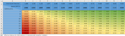
Using the Chart

In the chart above, I have added a row for the clock cycle time at each given speed, which, since this is DDR RAM, is 2000/speed. This is just for informational purposes.

The effective latencies are color coded using the “conditional formatting—graded color scale” feature of Excel. Latencies that are the same have the same background color, with green being the lowest latency and red the worst.

You will notice that most speed values in the column header are in bold. These speeds are approximately divisible by 266 MT/s, which is 133 MHz, since this is DDR RAM. More specifically, they are multiples of 133 ⅓ MHz rounded down to the nearest integer. These are the most common speeds, as they are multiples of the core clock speed used in computer circuits. But the reason I put them in bold has to do with overclocking. It happens that, as you take whole steps up in speed, you will also take a single step up in latency to get approximately the same true latency. For example, if I have DDR RAM rated at 1866 MT/s and 7 CL, you will see in the chart that the effective latency is 7.50 ns. If I want to overclock that memory to 2133 MT/s, which is one bold number higher, I should initially add 1 to the CL value, setting it to 8, which you will see in the chart is also 7.50 ns. With memory overclocking, once you find the highest stable speed, you can then attempt to lower the latency. The reason for always doing it in that order will be more apparent after reading the Burst Transfers section below.

If you are forced to lower the speed of your existing memory due to motherboard limitations, you can also lower the CL value so that you will end up with a similar value for effective latency. Either use the chart or count the number of speed jumps.

You can also calculate a new latency value using the following formula and rounding up:

• New CL = original E * New D / 2000

To avoid using the chart, this equation can be simplified as follows. I’ll use an apostrophe to represent the new latency (L’) and the new or required data transfer speed (D’).

1. Rewrite above equation:
   L’ = E * D’ / 2000
2. Remember that E = L * 2000 / D:
   L’ = L * 2000 / D * D’ / 2000
3. The 2000’s cancel out:
   L’ = L / D * D’

So, take the memory’s latency value divided by its data transfer rate and multiply that with the required data transfer rate to get the new latency value. Round up if necessary to match a value allowed by the motherboard.

Burst Transfers

Burst transfers occur when the CPU is able to keep the queue of memory requests full. The subsequent memory prep that happens during latency occurs while the previous memory request is still being processed. So, during a burst transfer, only the initial latency and the data transfer rate need to be considered for calculating the total transfer time. Thus, for two chips with the same E (effective latency), the one with the higher D (data transfer rate) will be faster overall.

An improved way to gauge the overall speed of a memory card is to look at the total time to access 8 words in a burst transfer, as in the chart below. You will notice in the chart below that when you make a whole jump up in speed and raise the latency by one, you get a lower total time, even though the previous chart showed the same or similar effective latency.

click chart for larger view.

For example, if you have DDR RAM rated at 1866 MT/s and 7 CL, the total time to fetch 8 words is 11.25 ns. Going up one whole jump in speed to 2133 MT/s at 8 CL gives a total time of 10.78 ns. It is clear that the faster RAM with the higher latency is faster overall given that the effective latency is actually the same. If, on the other hand, the 2133 MT/s RAM has a CL of 9, then its total time of 11.72 ns is longer than the “slower” memory for a short burst transfer.

The calculation for Total Time in the gradient area of the chart is as follows:

• T = L * 2000 / D + 7 * 1000 / D

In words, Total Time = Effective latency + 7 * Data cycle time. As mentioned at the end of the Clock Cycle Time section above, remember that data cycle time is 1000 / D, which, for DDR RAM, is half the clock cycle time. Both clock cycle time and data cycle time for each memory speed have been included in the chart above. 7 is used in the calculation instead of 8 for 8 fetches because the data cycle time for the first fetch occurs during the latency time.

The above formula can be simplified to:

• T = (L * 2000 + 7000) / D

You can get a copy of the Excel file with the two charts →here←. The header labels will not display correctly in Google Drive, so you must download and display in Excel.

Building the Charts

It is not obvious to most people about how to create the gradient and diagonally split corner label used in the charts. I have written two articles explaining exactly how this was done using the first chart above as the example.

To learn about the gradient type of conditional formatting, please see my article on Using Gradients to Correlate Data.

The diagonally split corner label is not a built-in feature of Excel. To create this in your own spreadsheets, see my article on Dual-label Corner Cell (splitting a cell diagonally) or download the Excel add-in at code.barr.rocks.