Excel - Dual-label Corner Cell (splitting a cell diagonally)

It is hard to believe that Excel still doesn't have the built-in ability to display a cell split diagonally with independent labels in each half. There are several ways to solve this manually but with issues. The two main issues are that resizing cells can mess up some solutions and most solutions do not allow you to color each half independently.

This article demonstrates two complete solutions - one is an add-in that I built and the other is a manual process to do the same thing.

Summary

It is hard to believe that Excel still doesn't have the built-in ability to display a cell split diagonally with independent labels in each half. There are several ways to solve this manually but with issues. The two main issues are that resizing cells can mess up some solutions and most solutions do not allow you to color each half independently.

This article demonstrates two complete solutions - one is an add-in that I built and the other is a manual process to do the same thing.

Why do we need this

Microsoft, are you listening?

In many tables, the purpose of the values in both the row and column headers is obvious, so you don’t need to label them. In most other tables, only the row header—or more rarely, the column header—needs to be labeled.

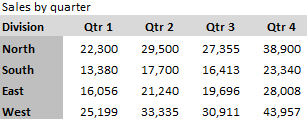
For example, the table below displays sales by quarter. Not only does the column label “Qtr 1” not need to be explained, but any label you added would likely be redundant. On the other hand, the fact that North, South, East and West represent divisions and not, for example, regions, is not so obvious.

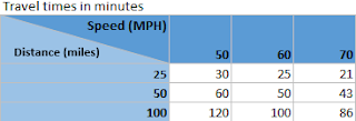
But what do you do when both the column header and the row header need a label? This was the issue I faced when writing my article on RAM Latency VS Clock Speed. In the spreadsheet below, both the row header and column header cells are used in the formulas in the grid and are just numbers. Both headers need to be labeled.

click to view entire chart.For information about creating the gradient in this image, see my article on Using Gradients to Correlate Data

The Easy Solution (extending Excel)

I have written an Excel add-in (free and with source code) that adds a toolbar button for turning a cell into a diagonally split cell. The button opens a dialog box that allows you to independently set the properties for each half of the cell.

click to view actual size.

The easiest way to use this feature is to create the row and column headers first with the desired background colors and fonts. Then select the corner cell and click on the Diagonal Split button that has been added to the toolbar. The dialog then opens pre-filled with the format properties of the existing row and column headers.

If you later make changes to the header formats, you can use this dialog to copy those changes to the appropriate half of the corner cell. There is no Save button on the dialog because each change is made immediately. This lets you try different settings and see the result at the same time.

Hovering over any of the controls on the dialog will provide a tooltip at the bottom left of the dialog.

My github page with the link to the add-in is here._↩

The Manual Solution

If I hadn't already written this section in a previous white-paper, I wouldn't include it now. It is a lot of steps.

To create two independent cell sections cut by the diagonal, we will insert two right triangles, with one rotated 180°. If you leave the borders on the triangles, they will overlap and not look right. But if you hide the borders, there will be a gap between the triangles. To solve this, start by setting the background color of the destination cell to match the color of the column header. While you’re at it, now is the time to set a diagonal border in this cell if you want one.

The instructions for the triangle that contains the row header label will be more straightforward and will be first:

1. On the Insert tab, click the Shapes dropdown and select the right triangle.
   
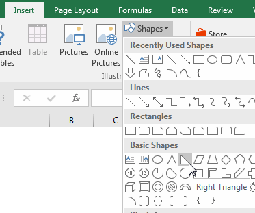
2. Draw the triangle by dragging the crosshairs from the top left corner of the destination cell to the bottom right corner. Holding down the {Alt} key while dragging the crosshairs will cause the object to perfectly align with the cell borders.
   
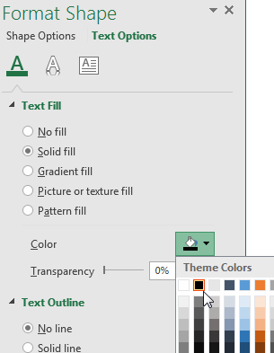
3. Right-click on the shape and select “Format Shape…” to bring up the Format Shape panel. From there you can change the fill color to match the row header. Also change the Line to “No line.”
4. Still using the Format Shape panel, go to Text Options. The default color for text is white. I have changed that to black in my example.
   
5. Select the Textbox icon and make the following changes:
   
   
   1. Vertical alignment: Bottom
   2. All margins: 0
   3. Wrap text in shape: Unchecked
6. Now just type the label text. With the object selected, the text you type will be part of that object.

Getting the column header label to look correct takes a bit more effort:

1. Draw another right triangle right on top of the previous one. Remember to hold the {Alt} key while drawing.
2. Right-click on the shape and select “Format Shape…” to bring up the Format Shape panel if it isn’t already displayed. This time, change the fill color to match the column header and again change Line to “No line.”
3. Click on the Effects icon and make the following changes under 3-D Rotation:
   
   
   1. Y Rotation: 20° (This tweak has the effect of shrinking the object horizontally just enough so that the shape does not cover the cell’s top and bottom borders. This is easier than trying to adjust the height and position.)
   2. Z Rotation: 180°
   3. Keep text flat: Checked (This keeps the text from following the object’s rotation, which, in this case, would have made it upside down.)
   
   Do not try to use other methods for rotating the shape. If you use the rotation handle or the Rotation value on the Size & Properties page, the text you enter will be upside down. Interestingly, the rotation handle doesn’t display if you are near the top of the spreadsheet area in Excel.
4. Go to the Text Options page and set the text color if necessary.
5. Select the Textbox icon and make the same changes as with the first triangle:
   1. Vertical alignment: Bottom
   2. All margins: 0
   3. Wrap text in shape: Unchecked
   
   Because the shape is upside down, its bottom is actually at the top of the cell. So setting alignment to the bottom will put text in the widest part of the shape.
6. Click on the shape and type the desired label.

Given the number of steps this requires and the care that must be taken if you want to change it later, you can see why I took the time to create the add-in.